In this post, I introduce the basic combinatorics that anyone who is serious about statistics beyond the most basic level should know. This part of math also, I think, happens to be exceptionally beautiful.

The lay of the land

The question “how many ways are there of choosing \(k\) items from a set of \(n\)” is a question that comes up constantly in mathematics.

To answer this question, we need to realize that there are actually four general situations where we can think of what we’re doing as “choosing (k) items from a set of (n)”. These can be represented on a \(2x2\) matrix. One dimension of variation is whether or not we can replace items after we pick them. Another dimension of variation is whether or not we care about the order in which items are picked. See below; each cell gives the “term of art” for the situation formed by the intersection of the column and the row. These notes focus on situations without replacement since they are generally more common in some areas of applied math.

Counting without replacement

To understand the two most important situations—where we do not have replacement—let’s suppose that we are members of a hockey team with six members.

Permutations without replacement

Let’s suppose that we are first interested in a silly situation, taking the team’s photo for promotional material. How many different orders can the team stand in? After a little reflection, we see that in the first slot, we could put any of six people, but once we do that, there are only five people available for the next slot, four for the next, and so on. We have \(6! = 720\) (which is mindblowingly large, I think).

We generally refer to this situation as a permutation, where this means that the order of selections matters. The way to remember this is a dumb joke: your bike’s combination lock is actually a permutation lock.

Now, we took a very easy case just now. We had \(n = 6\) people and selected all \(k=6)\) of them. What if ask after how many ways we could line up three members (for whatever reason)? Then, it is clear that we just want the first three terms of the factorial. This turns out to be easy to write more simply, even though factorial arithmetic is generally resistant to easy simplification. We can simply divide \(6!\) by \(3!\), leaving only \(6\cdot5\cdot4\). This generalizes easily. Defining \(nPk\) as the number of ways to permute \(k\) items taken from a set of \(n\), we have:

Let’s build a bridge case to the next question. Let’s say we now want to pick a first captain and second captain for our team. This is also solved in the same way, although it may not be obvious. However, to get the intuition, imagine writing “first captain” and “second captain” on slips of paper and putting them on chairs. Now, imagine all of ways you can pick two people to sit in these two distinguishable chairs. This is clearly \(6P2\): we have six people available to pick for first captain and five after that.

Combinations (without replacement)

Now, let’s change our question slightly. Let’s examine the number of ways to select a group of, say, two captains from our team. There are several good ways to think about this question. The first is that we could reason as follows. Our old formula (nPk) works quite well to count the number of ways we could pick a first captain and a second captain” because, in that scenario, we distinguish the two. However, if we only care about the group of people who are captains, note that our formula overcounts! By what factor does it overcount? Well, we can reason that, because we’ll eventually get every possible ordering of any distinct group of \(k\) people, it overcounts each group of people by however many ways that they can be rearranged, which is \(k\) as we saw from before.¹

This generalizes easily. Defining \(nCk\) as the number of ways to pick \(k\) items taken from a set of \(n\), we have:

Some subtleties in the permutation/combination relation

Note, by the way, that we could also see the problem a bit more generally in a way that will be useful later. Imagine that we simply mark our two captains chairs and put them together with four non-captain chairs. Now, we just find all the rearrangements of the team into the six chairs (\(n!\)) and deflate our count by the nuisance rearrangements of captains (\(2!\)) and non-captains (\(4!\)). This yields the same answer. In fact, the permutation coefficient can even be seen in this light, although we derived it differently above: we do care about order within our group of interest, just not in the “out group”, so we simply count all orderings of the total (\(n!\) and then divide by the spurious permutations of the out-group, \(k!\). And, finally, you may want to realize that the binomial coefficient doesn’t, strictly speaking, ignore order, but it instead simply ignores order up to group membership: it counts the number of ways that you could have a sequence of classes. You might want to keep the simple example in mind of a gym class with boys and girls, as those often line up “boy-girl-boy-girl” for activities. If your gym teacher is interested in all of the possible such class permutations, even the silliest ones (e.g., \(10\) boys, \(2\) girls, \(2\) boys, \(10\) girls, or something), this is what the binomial coefficient counts.

Finally, note that the limit cases all do what we would expect. Logically, \(\binom{n}{0} = \binom{n}{n} = 1\) (verify this algebraically) since there is only one way to pick everyone or no one; \(\binom{n}{1} = \binom{n}{n-1} = n\) (verify this algebraically) since it is obvious that to pick one person, or everyone but one person (i.e., picking one person whom to leave out), we have \(n\) choices.

Key facts about the binomial coefficient: symmetry

Algebraically, the binomial coefficient \(\binom{n}{k} = \binom{n}{n-k}\) (the reader can verify this). But, just as important, conceptually a binomial coefficient gives the number of ways to pick \(k\) items from a set of \(n\). But, if any way of choosing (k) items from a set of \(n\) leaves \(n-k\) left over, then every single way of picking of \(k\) items is a way of “picking” \(n-k\), so they logically have to hold up. After all, if you picture, say, an unsolved puzzle on the table, one way to “pick” \(k\) pieces is simply to lay a length of twine down the table, separating it into \(k\) and \(n-k\) parts (by definition since you must have \(n\) pieces for some appropriate choice of \(n\), e.g. 1000). I’ll explain why this is called “symmetry”, specifically, in a moment.

Key facts about the binomial coefficient: Pascal’s triangle/paths

Have you ever seen or constructed by hand Pascal’s ² triangle? This is easy to do by hand. We start with the arbitrary number one, a buoy floating atop a sea surface of zeros (not pictured below; I’m using the standard picture). Then, you can form any number in the triangle by adding together the two numbers directly above it. Remember that there are zeros everywhere outside the triangle.

How is this in any way connected to the binomial theorem? Well, all of those numbers in the triangle are binomial coefficients for \(n = \text{row number}\) (starting at zero, please note!) and \(k = \text{“column” number}\).

Now, why is this true? There are a few connections. ³

Let’s spell these out formally using induction. Proof by induction requires two steps. First, we prove or assume that something is true for a “base” case, such as \(n=0\) (if we’re, say, doing something like working out the closed form for a sequence). Then, we prove that if something holds true for \(n\), it holds true for \(n+1\). I’ll call these the “base case” and “generic step” moves below. Finally, these two things, taken together, imply that our claim is true for all positive \(n\). A common metaphor for this is that of the “ladder”: if I can prove that you can get onto a ladder in the first place, and that from any rung you can make it to the next one, this proves that you can go arbitrarily far on the ladder (note that this is obviously unrealistic in the real world; it useful to consider the reason, which is that we could never truly prove, for a finite human being, that they can get from any rung to any other without referring at all to their fatigue).

Here, we’re using induction in a sort of meta way. Our goal specifically will be to establish that, given the existence of two triangles with two different starting assumptions, the only way to get the items in each triangle is the same, and thus the triangles must correspond. So, in other words, we have a known rule for the classic triangle, which I’ll call generic step 1. Then, we show that the rule for the other triangle is equivalent (I’ll call this generic step 2). As long as the triangles start with the same numeric value, they are therefore numerically the same, and as long as the initial value can be represented as a binomial coefficient (things we establish in the base case step), then the two triangles are just different representations of the same thing, which is what we want to prove.

Base case: Assume that two triangles exist. The first is just the regular Pascal triangle. The second is a triangle fully of lily-pads, arranged like Pascal’s triangle, which a frog can hop between. From the first lily-pad, it can hop down and to the left, or down and to the right. On each lily-pad, we write down the number of ways to get to it from the first lily-pad. The frog can’t hop into the water on either side, so it must make at least zero hops to the right (i.e., \(n\) to the left) and no more than \(n\) hops to the right.

Generic step 1: To sum up the number of ways to get any place, in a very general sense, it is sufficient to sum up all of the ways to the “gates” of the place. For example, the gym I attend can be by several different doors. If those “gates” to the gym are the only ways to get into the gym, then the number of ways to get to the gym is the sum of the ways to end up at those gates. This is true for both triangles: obtaining any element by summing up the two elements directly above it is the most basic way to form the “classic” triangle, but it also must be true for the “lily pad” triangle.

Generic step 2: The frog must hop down \(n\) times to get to row \(n\), and since it can only move right while also moving down, that means that \(k\) of those \(n\) hops must also be down and to the right. Thus, the number of ways it can get to any lily-pad is \(\binom{n}{k}\).

So, we conclude that the number of ways to get to any spot on the lily-pad is both the sum of the two gates into it (so, it is the same as the Pascal triangle) and \(\binom{n}{k}\) (so, it is the binomial triangle).

Key facts about the binomial coefficient: Pascal’s rule

The second way is also very interesting. It uses more directly a fact implicit in the last example, a fact called “Pascal’s rule”⁴: \(\binom{n-1}{k-1}+\binom{n-1}{k} = \binom{n}{k}\). In words, this says that to find the number of ways to pick \(k\) items from a set of \(n\), we simply find the number of ways to pick one fewer item from a set of one fewer item and add this to the number of ways to pick fully \(k\) items from a set one size smaller. I’ll prove this in a moment; for now, just notice that this means that the entries in the binomial representation of the triangle can be now interpreted as the sums of the “parent entries”, at least before we get to the (arbitrary/mystical) first element.

Let us again use induction and prove that two triangles, the classic Pascal triangle and a new one, obey the same rules.

Base case. Assume that we start with, in the first triangle, a row of \(0\)s (arbitrarily long) with a \(1\) in the middle, \(…0, 0, 1, 0, 0…\). Assume that in the second triangle we start with a row of binomial coefficients, \(…\binom{0}{-2}, \binom{0}{-1}, \binom{0}{0}, \binom{0}{1} \binom{0}{1}, …\), which are equal to \(…0, 0, 1, 0, 0…\) logically (there are no ways to choose \(<0\) or \(>n\) things from a set of \(n\).

Generic step 1: In the classic triangle, any element in row \(n\), column \(k\) is the sum of the element in row \(n-1\) and column \(k-1\) with the element in row \(n-1\) and column \(k\) (this is just a slightly formalized description of how we introduce this triangle to kids, with nothing fancy really happening). Any element is the sum of its two “shoulders”.

Generic step 2: Any binomial coefficient \(\binom{n}{k}\) is equal to the sum \(\binom{n-1}{k-1}+\binom{n-1}{k}\), which we’ll prove shortly. So, if two adjacent elements in the triangle are interpretable as \(\binom{\text{row}}{\text{column}}\), and we form the element below and between them by summing them, that next element is also interpretable as \(\binom{\text{row}}{\text{column}}\).

So, we conclude that since we were able to validly represent the first row of the Pascal triangle as binomial coefficients with \(n = 0 = \text{row number}\) and \(k=\text{column number}\), and since this is true for any element in the triangle where we’re willing to grant that its two “shoulders” are binomial coefficients \(: \binom{\text{row}}{\text{column}}\) and we form it by summing the shoulders, the “binomial triangle” is just the sum of its two shoulders. So, the two triangles will always be the same.

So, then, why is Pascal’s rule true? There is an algebraic proof, but it is far less interesting than the logical proof. Imagine that the Mystery Inc. gang—Fred, Daphne, Velma, Shaggy, and Scooby—decides to split up to go look for clues. They are trying to decide who will investigate the abandoned amusement park and decide to send three people no matter what. At first, Fred says “I’m reading on this map that there’s some noshable kibble there!” Scooby perks up: “count me in for sure!” Velma reasons clearly that now they only need to pick two people out of the remaining four: \(\binom{4}{2}\). Then, however, she looks more carefully at Fred’s map. “Fred, you dolt!” she exclaims. “It says that there’s a nefarious cabal there!” “Zoinks!” says Scooby. “Count me out no matter what!” The gang now reasons that they now need to choose all three people from only four: \(\binom{4}{3}\). Then, however, Daphne takes a look at the map, and notices that the map is all smudged and it’s not really clear what it says, so that they might as well stick with the original plan. “Jinkies”, says Velma. “This is getting hard to count”. Shaggy, in a rare moment of lucidity, points out that if they are considering all search parties of size three with Scooby definitely included (\(\binom{4}{2} = \binom{n-1}{k-1}\) from before) and all search parties of size three with Scooby definitely excluded (\(\binom{4}{3} = \binom{n-1}{k}\) from before), their sum can’t possibly differ from the number of search parties that can be formed of size three using all five members (some include Scooby, some don’t; all five members are candidates): \(\binom{5}{3} = \binom{n}{k}\). This completes the proof.

Finally, we can return to the question of symmetry mentioned above. Why do we call the fact that \(\binom{n}{k} = \binom{n}{n-k}\) the property of symmetry? Well, if we folded Pascal’s triangle in half, we’d see that the two coefficients would line up: (\binom{n}{k}\) is \(k\) steps in from the right, while \(\binom{n}{n-k}\) is \(k\) steps in from the left.

Key facts about the binomial coefficient: the hockey stick identity

Now we can prove another cool fact about Pascal’s triangle. Note that we can form a series of binomial coefficients through the triangle that resemble a hockey stick. The terms in the “handle” sum to the (short) “blade”.

Why is this so? The key is to see this combinatorially (i.e., logically), rather than working through a tedious algebraic proof. Return to the Scooby Doo example.

Imagine that the Mystery Inc. gang (four people plus a dog) wants to split up. One group will look for clues; the other will stay behind. They want to make the clue group larger, of size \(3\), so we want to find \(\binom{5}{3}\). Suppose we designate a subgroup of two of them, Shaggy and Scooby, to be unreliable when looking for clues alone. So, we think about the process of picking the clues group as ensuring that there is at least one “responsible person” in the group. We start with Daphne and count all groups involving her and two other people, whether or not this includes Shaggy and/or Scooby: this is \(\binom{4}{2}\). It is worth recalling that we derived this fact above: if we have \(n\) people and want to pick a group of \(k\) that definitely includes person \(i\), then we must count \(\binom{n-1}{k-1}\) because we have one fewer person to choose from (\(n-1\)) but we also only need \(k-1\) people because we know that person \(i\) will complete the group.

Then, we do the same for all groups involving Fred. Daphne is already spoken for, so this is \(\binom{3}{2}\), by a similar argument: we now omit two people from consideration (Daphne: already counted; Fred: must be involved, so we disregard him). Finally, Velma can be involved in only one way that we haven’t already counted, which is is her serving as Scooby and Shaggy’s chaperone. This leaves only \(\binom{2}{2} = 1\) group of counterparts for her. Finally, there is no need for Shaggy and Scooby to count their groups because they can’t form one without involving at least one of the leaders, and all the leaders have counted so far. Note that this is true even without the little narrative conceit of “leaders”; they are also not enough people!

Let’s try to generalize the story a bit. We want to form a group of size \(k\); one way to do this is to split our larger group into \(k-1\) elements designated “followers” and \(n-(k-1)\) designated “leaders”. Logically, any possible group needs at least one person from the leader group; the largest possible group of only followers is still too small. So, if we could find a way to find partition all groups that are large enough into those definitely involving leader \(1\), then those remaining groups which definitely involve leader \(2\), etc., we would come up with the number of the possible groups. Then, generically, a group of \(k\) from a group of \(n\) that definitely includes someone can be formed \(\binom{n-1}{k-1}\) ways; then, the number of groups excluding person \(1\) and including person \(2\) must subtrac them both from consideration: \(\binom{n-2}{k-1}\). Then, we simply iterate until we get to the smallest possible group: this would be a group that accounts for all \(n-k+1\) leaders, i.e. \(\binom{n - (n-k+1)}{k-1} = \binom{k-1}{k=1}\). Again, this logically must exhaust all possible groups: we can’t get a group of \(k\) from a group of \(k-1\) using any kind of sorcery. Using summation notation and the dummy parameter \(j\), we are asserting that \(\binom{n}{k} = \sum_{j=0}^{n-k} \binom{n-j-1}{k-1}\). (Note, by the way, that we did not use, here, the other interpretation of Pascal’s rule, that going “up and to the right” means ensuring that one person is not in a group of the same size; there is a way to form this interpretation, but it is less direct). In other words, once we start on the “blade”, we move up and to the right because we are reducing our population size by one each time and thereby ensuring that multiple successive people are included in the group.

Key facts about the binomial coefficient: counting the sum of the first positive \(n\) integers

Here is another beautiful connection that I don’t see mentioned very often. How can you sum the first \(n\) positive integers? First, let’s prove it in the standard way.

To find the sum of the first \(n\) positive integers, note that \(S_n = \sum_{i=1}^n i\) can be doubled so that we have \(2S_n = \sum_{i=1}^n i + \sum_{i=1}^n (n-i+1)\). Then, …

This is a (less beautiful) summation-notation version of a beautiful proof that works better on a blackboard that Gauss allegedly arrived at when he was only seven (thanks to the terrific Art of Problem Solving book for this proof and anecdote, although Weissman reports in An Illustrated Theory of Numbers that the ultimate source for this claim is much less bold).

Note that this can also be arrived at entirely independently by means of the binomial coefficient. Consider the question—posed to me first by my wonderful third-grade math teacher Ms. Ball—“how many unique handshakes can be made among members of our class?”

The simplest answer (one that I did not grasp at the time, but one which seems trivially obvious now) is to apply the above approach. Start with an arbitrary person \(1\), who can shake everyone else’s hand but his own; then, person \(2\), who can shake everyone else’s hand but person 1’s; and, so on. We end with person n, who cannot shake anyone else’s hand, for everyone else has shaken his. Thus, the task is to find \((n-1) + (n-2) + … + 1 + 0\). This is equal to the sum of the first \(n-1\) positive integers, and our formula above tells us that the answer is \(\frac{n(n-1)}{2}\).

To my credit, I remember finding this problem confusing because I wanted to take the combinatorial approach, which is too difficult to make much headway with at that age. However, the problem is simple for a talented high school student. How many unique pairs are there of two people in a group of \(n\)?

First, overcount it: find out how many ways there are to order two people out of the (n). This is easy; we can start with each person, and then we end up with one person fewer with whom to pair them, so we have \(n\cdot(n-1)\), which can be written for the sake of generalizing as \(\frac{n!}{(n-2)!}\).

Then, we realize that this formula overcounts by the number of ways to order the group of size \(k\) which we select: each permutation of size \(k\) given by the formula \(\frac{n!}{(n-k)!}\) is a member of a group with all the same elements, just arranged in a different order; since each permutation is of the same “length”, every unique group is overcounted by a factor of \(k!\), so the formula for the sum of permutations overcounts the sum of groups by that exact factor. So, if we just divide by the old formula by \(k!\), we’ll have ready to hand the desired quantum.

Here, we obtain \(\frac{n(n-1)}{2}\), which is the same formula we found above for the sum of the first \(n-1\) positive integers. To add the \(n\)th term, we simply add \(n\) to the formula (multiplying by two because the whole thing is divided by two), which we can do easily with multiplication by changing the \((n-1)\) to \((n+1)\). The answer follows.

The binomial theorem

A more general use of the binomial coefficient is in the binomial theorem.

Logic of binomial (and multinomial) expansion: the box method reviewed, “why FOIL works”

First, note that the binomial coefficient given above is helpful in writing the binomial expansion (after all, that is why it is has a special name that, at first, appears to be unrelated to its combinatorial meaning).

If we have the expansion \((x+y)^n\), we can write the product as \((x+y)_1(x+y)_2…(x+y)_n\). Based on the validity of the “box method” of multiplication, we can see that in two and three dimensions, to get the area or volume of a square (or cube) with each side partitioned into \((x+y)\), we start with the first dimension, denoted \((x+y)_1\) above, and find all the unique combinations of \(x_1\) with every element from the other sides (e.g., if we have three dimensions, we would need \(x_1\cdot x_2 \cdot x_3\) and \(x_1\cdot x_2 \cdot y_3\) and \(x_1\cdot y_2 \cdot x_3\) and \(x_1\cdot y_2 \cdot y_3\). To go further, you can either conceptually consider a box in \(n\) dimensions or simply work iteratively in two dimensions; e.g., after working out the rule for a square in two dimensions, write a new rectangle (not a square) with one side partitioned into \(x^2 + xy + xy + y^2\) and the other into \(x + y\) alone; this represents cubing. You can then write the result of the cube on the side of a new rectangle and the other as \(x + y\) alone, representing the power of 4, all without resorting to higher dimensions.

The pattern that we find is that \((x+y)^n\) is formed by taking the product \((x+y)_1(x+y)_2…(x+y)_n\), going “bucket by bucket”, and selecting \(x_i\) or \(y_i\) from each bucket until we exhaust all possible combinations (note that order does not matter here; we do keep track of which bucket we pull an \(x_i\) from, hence the subscript, but we don’t care about the difference between, e.g., \(x_1y_1\) and \(y_1x_1\)).

For what it’s worth, this is identical to saying that we want to let some index \(k\) vary from \(0\) to \(n\) and then find all combinations of \(k\) terms of \(x\) (or \(n-k\) terms of \(y\)) from the \(n\) buckets. That is, there are \(\sum_{k=0}^n \binom{n}{k} = 2^n\) terms formed in this way because this is also equal to the number of permutations with replacement from \(n\) repeatable “trials” on a coin labeled \(x\) and \(y\).

The binomial theorem: using the binomial coefficient to generalize the box method for taking a binomial to the \(n\)th power

All of that last paragraph is somewhat besides the point. All we need to do is realize that each term formed this way must be of the form \(x^ay^b\) for some \(a, b \geq 0\). Then, we realize that from \(n\) buckets, if we can choose \(k\) to be \(x\), this means that there are \(\binom{n}{k}\) ways to select a term with \(x\) multiplied \(k\) times, i.e. \(x^k\). Note that we don’t need to worry about the \(y\) term directly. This is because the binomial coefficient is symmetric (per the above), so the number of ways to pick \(k\) \(x\)s from \(n\) “buckets” is also the number of ways to pick \(n-k\) \(y\)s from \(n\) buckets.

So, our general formula is …

A quick motivation for the binomial theorem: proving the power rule

Let’s learn a very easy and useful part of calculus. One of the two big ideas of calculus is that we care a lot about non-linear functions, but the “speed” of such a function, its slope, varies, unlike linear functions. We often want to find rules about the rate of change at some particular value \(x\) in the very immediate vicinity. This “instantaneous rate of change” or “instantaneous slope” is called the derivative. That’s all there is to it! We define it (in modern terms) as \(\lim_{h \rightarrow 0} \frac{f(x+h)-f(x)}{(x+h) - x}\), the limit of our function’s slope for a tiny change in \(x\), here denoted \(h\), as \(h\) gets infinitely small. The problem in evaluating this is that the denominator simplifies to \(h\), so our regular limit trick of plugging in \(h=0\) won’t work directly. Fortunately, there are many fun workarounds.

The most commonly-used derivative rule in calculus works like this, in the simplest case. If we have some simple function \(f(x) = x^n\), then \(\frac{df}{dx} = nx^{n-1}\). How can this be proven? It’s actually extremely simple using the binomial theorem.

Now we can safely plug in \(h=0\) without fear of a zero in the denominator: \(\frac{d(x^n)}{dx} = nx^{n-1}\).

Permutations with replacement

These are pretty easy to describe. They typify certain cryptography problems. A good example is the number of ways that you can choose a code for your bike lock. Here, we can reuse digits. So, since we can have any one of 10 digits five times (if the lock is the standard length), we have \(10^5\). More generally, we have \(n^k\).

Note that in this case, by the way, \(n\) and \(k\) shift their meaning subtly. We have (n) opportunities to choose \(k\) outcomes, but it is not true any longer that \(k \subset n\), i.e. \(k\) does not have to be a subset of \(n\). Another classic example is the number of ways to flip a coin \(n\) times. Here, we have \(k = 2\) outcomes, but we could flip the coin once, twice, or three times; we do not require \(n \geq k\).

Combinations with replacement

These are sometimes also called multisets. These are written as combinations, but they are not, strictly speaking, combination-style questions. Let’s switch metaphors a bit. A concrete example is this: if I am at a barbecue joint and order a protein-packed dinner with \(k = 4\) servings of meat, which I can choose from \(n=3\) options (say, beef, chicken, and pork), the number of ways I can allocate my choices is given by \(\binom{n+k-1}{k} = \binom{n+k-1}{n-1} = \binom{6}{2} = 15\).

Here is why: imagine that I order by standing in front of each type of meat in the case and saying “a scoop, please” and then moving to the right, to the next meat, when I’m done. So, I’m taking two actions: saying “yes” and moving right. If I start at meat (1), I only need to move right \(n-1\) times to get to the end, and this means that there are \(n + k - 1\) actions to take, of which I can choose (n-1) to be rightward steps or (k) to be “yes”es. This type of explanation is sometimes called “stars and bars” after an older explanation in Feller (1966), where the two classes of object were \(\ast\)s and \(\vert\)s. Notice that in this scenario, the size assigned to each class (the three options) is not fixed. Notice also that we don’t distinguish the scoops themselves: what we pay attention to are who gets how many scoops.

The multinomial coefficient

Don’t confuse the multiset coefficient, the number of ways to pick \(k\) items from a set of \(n\) choices when we can repeat, with the multinomial coefficient. Multinomials are similar only in a very general way, that they involve the distribution of a set of choices into different classes. However, in the multinomial scenario, the distribution is fixed, or assumed, whereas the whole purpose of the multiset is to let it vary and count all such variations. Both problems are often described with “ball and urn” scenarios, whereas simple permutations and combinations without replacement often use more palatable examples involving people, maybe causing the two to be confused.

The multinomial coefficient instead counts the number of ways to take \(n\) distinguishable objects and distribute them in fixed proportions into classes \(k_1, k_2, … k_m\). In somewhat sloppy fashion, these \(k\)s are also typically used to denote the size of each class which is fixed here.

To use a slightly-stilted modification of our previous example—since these coefficients count different things, it is hard to find a scenario where both answer equally natural questions—suppose that I settle on two scoops of beef, one of chicken, and one of pork. The distribution is fixed. However, now the clerk has a choice of where to put the food in the takeout tray. The number of ways they can do that is \(\frac{n!}{k_1!k_2!k_3!} = \frac{4!}{2!} = 12\) in this case (ignoring the two \(1!\)s). We imagine the spots in the tray lined up. The clerk can put the scoops in any order they like, but we divide by \(k_i!\) for each \(i\) because it doesn’t matter to the naked eye if the scoops of beef would be swapped.

You can consider the multinomial to give you the number of unique permutations of a set of items distributed into types, where the number of each type is fixed and we can’t distinguish items that are the same type. The binomial can also be considered this way; if I am deciding how many ways I can pick two guys on my football team of \(11\) to be co-captains, this is the same as lining everyone up and then giving people slips of paper that say “captain” or “non-captain”, except I don’t care about the ordering within the slips.

Conversely, the multinomial can also be derived as the product of multiple binomials. Let’s try a harder word like barbell. We first ask how many ways we can choose \(k_1\) slots from a set of \(n\) to be, say, ls. Then, we ask how many ways from a set of \(n - k_1\) we can let be the \(k_2\) bs. In general, the pattern looks like this (eschewing the formal statement)…

At each step of selecting some specific \(k_r\), we divide by \(k_r!\) to get rid of the spurious permutations of identical items within that class, and we also divide by \((n - \sum_{j=1}^{r} k_j)!\) so that the permutation of of the \((n - \sum_{j=1}^{r-1} k_j)\) available objects only goes through the first \(k_r\) steps (just like how we derive the binomial).

Polynomial expansion or multinomial expansion

Finally, let me mention one property that will be very useful later on. As mentioned before, you might have learned in school the “FOIL” property, which tells us how to expand quantities such as \((a+b)(c+d)\). We then saw that an important situation occurs when we “FOIL” quantities such as \((a+b)^2\) because this can be expanded to quantities such as \((a+b)^n\), and we can describe these with the binomial theorem.

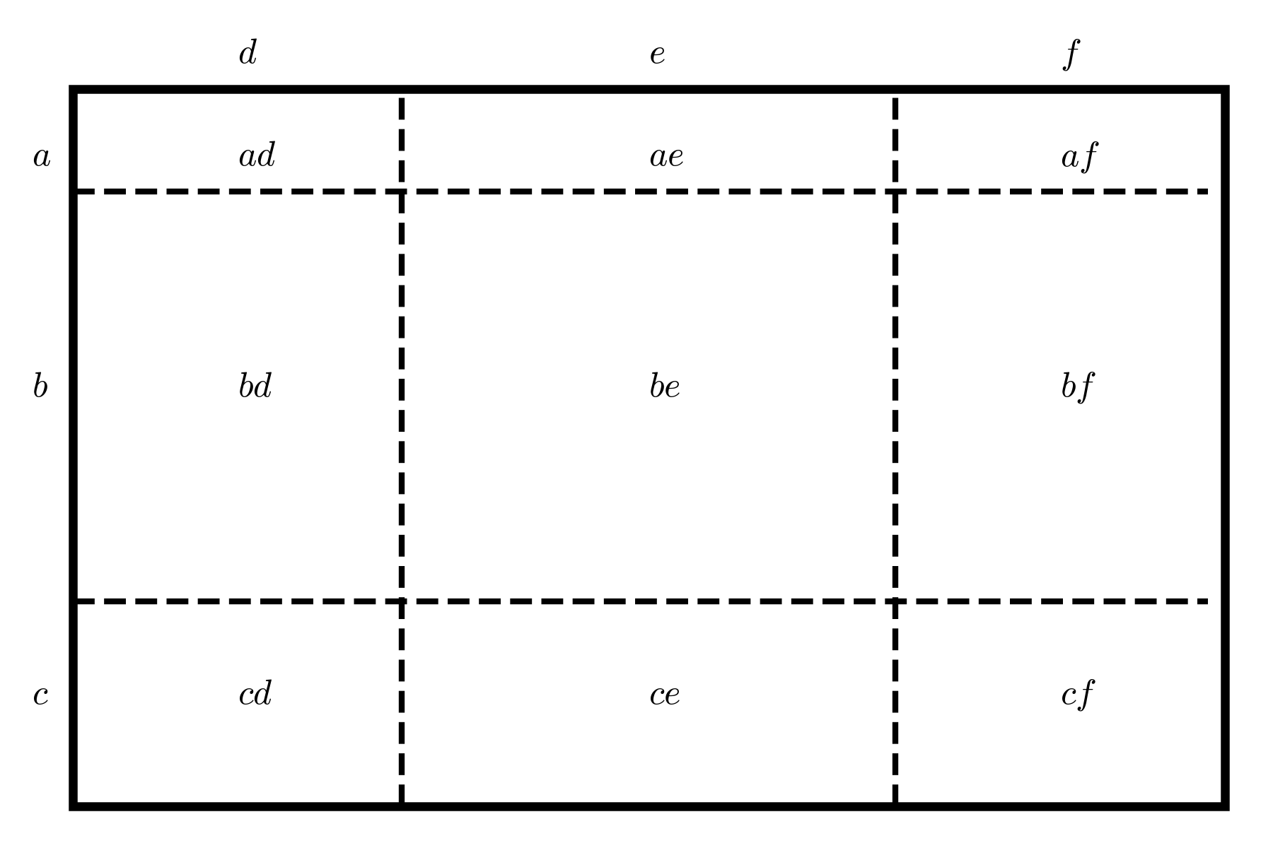
However, what if, instead, of incrementing the power of the binomial term, we tried multiplying together two polynomial terms? For example, how do we multiply out an expression such as \((a+b+c)(d+e+f)\)? Well, the solution, as it so often is in math, is to think geometrically about the problem. The graphic below makes quite clear, I think, how we ought to do this (I alluded to this method above, but here I think it is important to show it).

Now, let’s think about this quantity algebraically. It will often be convenient to write out multinomial expansion using summation notation. There are two useful ways to see this. First, imagine that we simply write out the product. Since we will often later want to refer to observations of a variable \(Y\) defined on a finite population, \(y_1, y_2, … y_N\), I’ll use that notation here.

Notice the following pattern. By starting with the left sum, picking a \(y_i\), and then moving through the second sum, we get \(y_i^2\) and then the product of \(y_i\) with every other \(y_j\). There is thus only one way to get any \(y_i^2\), but then any \(y_iy_j : i \neq j\) will appear twice, once when we start with \(y_i\) and once when we start with \(y_j\). We can write that in summation notation in two ways. First, we can just write that without mentioning the double-counting. We just say “sum all the squares from \(i=1\) to \(n\), then add all of the ‘mixed products’ \(y_iy_j\) for all values of \(j\) for any given \(i\) (skipping \(i=j\)), then do this for all values of \(i\)”. Translated into algebra, that is…

But, however, we can also include information on the repetition. one way to think about this is to say that we can just form all the unique products \(y_iy_j : i \neq j\) and notice that we have two of each. One way to do this when we use the notation of sums is to somehow “increment” our index variable for one of the sums (in the language of computer science”). What we would do is say “find all of the squares and set them aside”, as we already know how to say; then, we would say “fix a value of \(i=1\) and go through the \(j\)s that aren’t equal to \(i\), but for \(i=2\), start at \(j=3\) because we’ve already counted \(y_2^2\) when we counted the squares, and we already counted \(y_2y_1\) because we counted \(y_1y_2\) when we had \(i=1\); then, just multiply that double summation by two because we do in fact count it twice”. The specific way in which we translate this into a sum is that we say that we only want to count values of \(j\) that are greater than the current value of \(i\).

Translating this into an equation, we have…

Finally, notice that we often want to sum up the elements of a matrix such as the (variance) covariance matrix. This also provides a very nice picture of how this expansion works. Note that in the diagram below, the off-diagonal are counted twice (e.g., I have labeled both \(\sigma_{n1}\) and \(\sigma_{1n}\)). Further, we can easily refer to the upper-half of the matrix by saying that it is a place where the column number is larger than the row number (so, \(j>i\) if we let \(i\) index rows and \(j\) index columns). So, then, we just sum over all rows and columns with the restriction that the column number is greater than the row number, then multiply by two. Finally, we have to remember to add up all the elements on the main diagonal as well.

Bonus: Fibonacci numbers in the triangle

Edit 2024-04-25: I decided to add in the connection to Fibonacci numbers.

Fibonacci numbers

Fibonacci numbers are \(1, 1, 2, 3, 5, 8, 13, 21 … \), and they are written \(F_1, F_2, F_3…\). They are defined by the formula \(F_n = F_{n-1} + F_{n-2}\), except that \(F_1 = 1, F_2 = 1\) by construction. The sums of Fibonacci numbers are easy to work out because of this recursive property. We can avoid ugly restrictions on the index of numbers and simply write that \(F_{n+2} = F_{n+1} + F_{n}, n \in \mathbb{N}\) (where I follow the convention that zero is not a member of this set). This conveniently works for all \(n \geq 3\) and allows us to just define the first two elements by fiat.

The diagonals of a left-justified version of Pascal’s triangle sum to the Fibonacci numbers.

Below is how this looks on the regular triangle.

This property is actually relatively easy to explain. Here is an example.

On a trail I run, there are two loops, one coming to about a mile and the other about two. Suppose that I want to run five miles. How can we do this? I can run five of the one-mile loop, or a two-mile loop and then three of the one-mile loop (i.e. four total loops), or I can leave the two-mile loop for last, etc. In other words, there are many sequences of one- and two-mile loops that I can could run (we’ll count them exactly soon).

But, there is another way to count all of those ways to run five miles which connects that to the Fibonacci numbers: every possible way I have of doing this starts with either a one-mile loop or a two-mile loop. If one mile, then the remaining number of loops must sum to four miles; if two miles, then the remaining loops must sum to three miles. Thus, any way of running \(n\) miles is a sum of the ways to run \(n-2\) and \(n-1\) miles, just like in the Fibonacci formula. To work out the exact connection, we can put all this information into a table. Following Arthur Benjamin’s excellent book Magic of Math⁵ (to which I owe some debt), I will denote the number of ways to run \(n\) miles \(f_n\) and use \(F_n\) to denote the \(n\)th Fibonacci number. As we can see clearly, \(F_n = f_{n-1}\).

So, we have established the connection of our “sum of sequences comprised of \(1\)s and \(2\)s”. How do these two relate to binomial coefficients?

Well, working out the number of sequences that sum to \(n\) miles can also be understood as an exercise in asking “where do the \(2\)s, if any, go?” For example, for \(n = 5\), we can have \(0, 1,\) or \(2\) twos; the answer to “where do(es) the two(s) go?” is a binomial one, of course: asking about the number of ways to order \(m\) objects of type \(k_1\) and \(k_2\), where we don’t distinguish objects of the same type, is a classic way to re-describe the binomial coefficient as a multinomial coefficient as described above. Since we already demonstrated that the number of ways to sum \(1\)s and \(2\)s to get the natural numbers \(n\) is a Fibonacci sequence shifted, we now have the basic connection in hand.

Now, we work on the details. How many binomial coefficients do we need to sum up? Let’s start with the simplest scenario, which tells us where to begin the sum and also what our index variable should be: if we have no \(2\)s, we simply have \(\binom{n}{0}\). Then, if we just add in a \(2\), we would be incrementing the sum by by \(1\), so we have get rid of a \(1\); we have \(\binom{n-1}{1}\) places to put the single two.

Finally, where should we end our sum? Well, if we have an even number, we simply stop at \(\frac{n}{2}\), because \(\frac{n}{2}2 = n\). Then, the expression follows readily for even numbers:

Now, finally, we just need to work out what to do in the case of odd numbers. Here, we can just use hand-inspection. If \(n=5\), we can have, at most, a pair of \(5\)s, so we want the integer part of \(\frac{5}{2}\). This is denoted, at least in computer science, the floor of \(\frac{n}{2}\) and written \(\lfloor{\frac{5}{2}}\rfloor\) (note the little “feet” on the “bars”).

Finally, if we pick a given \(n\) on the “binomial triangle” and then simply run our finger along the triangle, we’ll see that this is always a diagonal of the triangle.